AP Physics Lab – Capacitors and RC Circuits

Purpose

Charging and discharging behavior of capacitors will be explored using various values for voltage, resistance, and capacitance. The theoretical functions for voltage and current versus time will be verified, as will the defining relation between capacitance, charge, and voltage.

Procedure

Part A – Basic RC Circuit

Voltage and current for the capacitor will be measured with Logger Pro 3. Construct the following circuit using appropriate connectors. Connect the current and voltage probes so that both will read positive values when the capacitor is charging. (The probes are shown as an ammeter and a voltmeter in the schematic.)

Connect the voltage probe to channel 1 and the current probe to channel 2 of the Lab Pro interface and connect the interface to the computer using the USB cable. Open the file “RC Circuit” in Logger Pro 3.

You should see live readouts of the sensors – try flipping the switch in the circuit to check for proper operation. Before proceeding you should zero both sensors by connecting a wire across the inputs of each sensor to ensure that the current and voltage are each truly zero and then click on the Zero button in Logger Pro. This is similar to using the Tare button on an electronic balance.

The file is set up to record the charging of a capacitor. Data collection is triggered when the voltage increases across 0.05 V (i.e. the voltage becomes greater than 0.05 V after being less than 0.05 V). Simply click on the Collect button and then flip the switch to charge the capacitor. If all goes well you should be able to produce smooth curves showing the voltage and current for the capacitor. (Tip: select a graph and click Autoscale to get a good view of all the data).

If you cannot produce graphs: check all connections, make sure the sensor is connected to register a positive voltage, make sure the capacitor is initially completely discharged. Also check the triggering settings and modify if necessary.

Once the system is working correctly create a set of graphs that clearly shows both charging and discharging during the allotted 2.0 seconds of time. This can be done by quickly flipping the switch from charging to discharging. Preferably the capacitor can be charged and discharged in about one second. You may have to make several attempts.

Data and Curve Fits

Use the analysis tools of Logger Pro to complete the appropriate parts of your data table.

q On Page 1 of the Logger Pro File: Charged Voltage can be found by using the Statistics button to find the mean value of the “final” charged voltage attained by the capacitor (select the “plateau”). Charge Input and Output can be found by Integration of selected portions of the current vs. time graph.

q Pages 2 and 3: The Coefficients can be found using an exponential Curve Fit of selected portions of the voltage vs. time and current vs. time graphs. Important Note: when doing the curve fits use the Time Offset option!

q Page 4: Resistances can be found by linear regressions of selected portions of the voltage vs. current graph.

Change the values of capacitance and resistance and repeat the process as needed to complete your data table for Part A.

Part B – Complex RC Circuit

Make the necessary changes to create the following circuit:

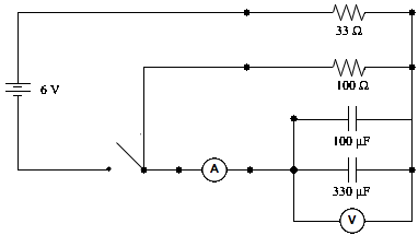
Analyze the results as you did in Part A, but this time print all four pages in landscape mode. Adjust the scales, labels, colors, and any other aspects of the graphs to get the best appearance and maximum usefulness for inclusion in your lab report.

Questions

1. Discuss whether or not your experiment supports the theoretical relations for capacitors and explain how so by referring specifically to tables, graphs, etc.

2. (a) Using your best judgment and all available data from the lab, determine a single
value of capacitance for each of the two capacitors based on the experiment.
(b) Determine the percent difference between each experimental value and the nominal value
printed on each capacitor. Show your work for both parts.

3. The voltage measured in this experiment was that across the capacitor. Explain why the slope of this voltage can be used to determine the resistance of the resistor for both charging and discharging in Part A. Is there any systematic error in this technique?

4. Do you think the internal resistance of the battery or the probes had a significant effect on the experiment? Support your answer with specific references to tables, graphs, etc.

5. Discuss the results of Part B – including specific consideration of both the charging and discharging. Evaluate any expected or unexpected outcomes. Make any appropriate numerical calculations and comparisons that would serve to evaluate how well the results support the theoretical behavior of the given circuit.

A complete report (50 pts): (6 or 7 pages in this order)

q Completed data/results tables. (8)

q Part B, Page 1: Data table and V vs t and I vs t graphs with statistics of plateau and integrals for charging and discharging. (8)

q Part B, Page 2: V vs t graph with exponential curve fits for charging and discharging. (8)

q Part B, Page 3: I vs t graph with exponential curve fits for charging and discharging. (8)

q Part B, Page 4: V vs. I graph w/ linear regressions for charging and discharging. (8)

q On separate paper, answers to the questions using complete sentences. (10)

Data Part A

		R = 100 Ω C = 330 μF	R = 10 Ω C = 330 μF	R = 100 Ω C = 100 μF	R = 33 Ω C = 100 μF
Statistical Mean of Plateau V vs t	Charged Voltage (V)
Integrals I vs t Charging and Discharging	Charge Input (mC)
	Charge Output (mC)
Coefficients of exponential functions V vs t	Coefficient Charging (s^–1)
	Coefficient Discharging (s^–1)
Coefficients of exponential functions I vs t	Coefficient Charging (s^–1)
	Coefficient Discharging (s^–1)
Slope of Linear Regressions V vs I	Resistance Charging (Ω)
	Resistance Discharging (Ω)

Data Part B

Printout of four pages showing statistics, integrals, and curve fits.

Calculated Capacitance based on Part A

	R = 100 Ω C = 330 μF	R = 10 Ω C = 330 μF	R = 100 Ω C = 100 μF	R = 33 Ω C = 100 μF
Calculation:	Capacitance (μF)	Capacitance (μF)	Capacitance (μF)	Capacitance (μF)
C = Q/V charge input
C = Q/V charge output
C = τ/R voltage charging
C = τ/R voltage discharging
C = τ/R current charging
C = τ/R current discharging
Mean Value of C
Mean Deviation

Show one example of each type of calculation used to complete the above table: